Marginalizing Multiplicative Noise Applied to Regression Predictors is Ridge Regression
Updated October 2026: Clarifies the distinction between the two ways to marginalize out multiplicative noise. The original post incorrectly averaged the lines, but only stacking recovers ridge.
Ridge penalization is a popular and well studied method for reducing the variance of predictions in regression. There are many different yet equivalent ways to think about ridge regression, some of the well known ones are:
- As a penalized optimization problem.
- As a constrained optimization problem.
- As a maximum a-posteriori estimate in Bayesian linear regression.
- As a linear regression on an augmented data set augmented with “fake” observations.
In this post we will describe another, less common, characterization of ridge regression.
Software
The code used to produce the simulations and plots in this post is available here.
Acknowledgements
The idea for this post was inspired by a small section in the paper: Dropout: A Simple Way to Prevent Neural Networks from Overfitting. After working this all out, I discovered a reference to the argument here in Efron and Hastie’s Computer Age Statistical Inference. The idea first appeared in Bishop, Training with Noise is Equivalent to Tikhonov Regularization.
Ridge Regression
Consider the usual regression setup with feature matrix $X$ and target variable $y$.
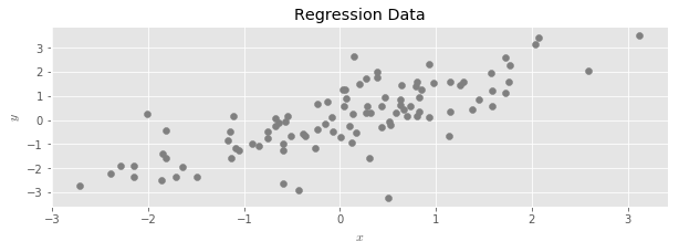
In linear regression, we seek a vector $\hat \beta$ which solves the following optimization problem:
The goal is to produce a linear function that can be used to predict new values of $y$ when only provided with values of $X$. Once $\hat \beta$ is obtained, these predicted values are given by:
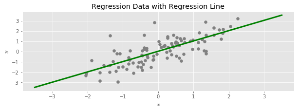
Ridge regression is an alternate way to estimate a regression line that is useful when linear regression produces predicted values with a high variance (for example, when there is not enough data available to accurately estimate effects for all of the available predictors). Ridge often has the desirable effect of improving the predictive power of a regression.
In the standard description, ridge regression is described as a penalized optimization problem:
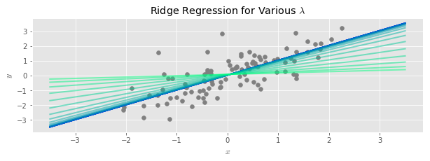
The parameter $\lambda$ controls the severity of the variance reduction: larger values attenuate the linear regression line more, and result in more biased but lower variance estimates.
Applying Multiplicative Noise to Regression Predictors
Suppose we have available an unlimited number of independent and identically distributed Gaussian random variables with mean one and standard deviation $\sigma$:
If $X$ is the matrix containing feature values, we say we have applied multiplicative random noise to X when we replace $X$ with:
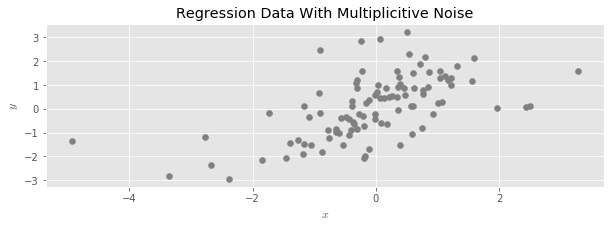
In words, we draw a random $N(1, \sigma^2)$ for every data element in $X$, and then multiply each data element by its corresponding random number. Here’s what that looks like:
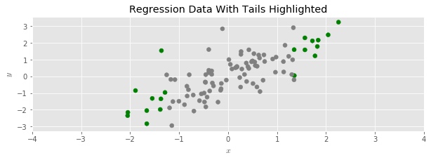
To see the effect more clearly, let’s color the upper and lower 10th percentiles of the example regression data set:
And then disperse the data with multiplicative random noise:
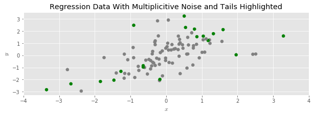
We see that the data has spread out, and its range has expanded; around half of the shaded points moved further away from the center of the point cloud. The idea is to fit a linear regression, but to the manipulated data. Intuitively, this should have the qualitative effect of attenuating the regression line, just as in ridge regression.
In the plot below, the original data set is plotted in black, and the dispersed data we used to fit the regression line is plotted in light grey. As more noise is applied, the regression line indeed flattens.
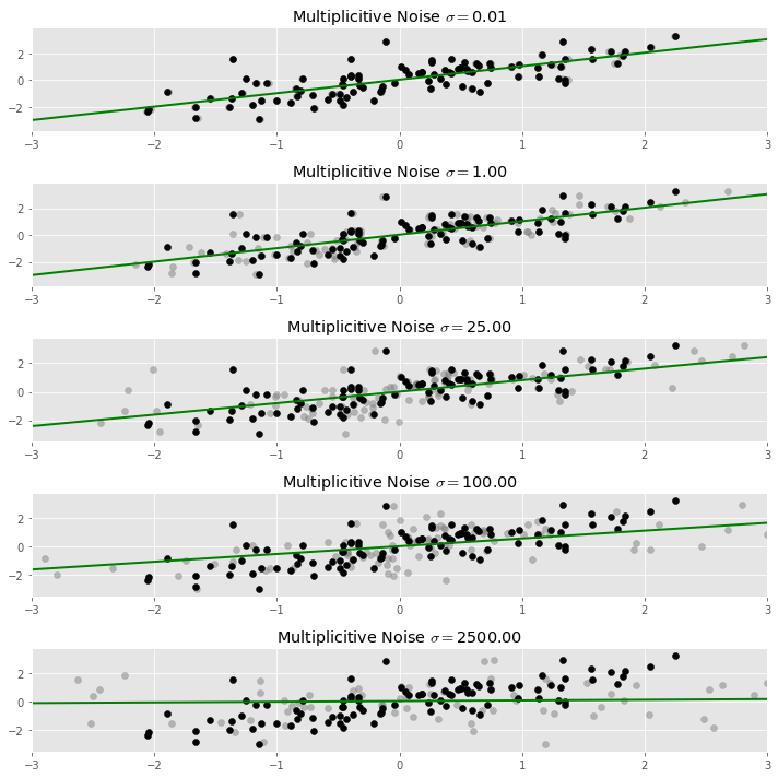
Of course, when applying random noise to data, one expects to get a different result each time. In our case, each time we fit a regression line to a different version of our noisy data, we expect to get a slightly different line. We would like to get a stable result out of this process, and there are a couple options:
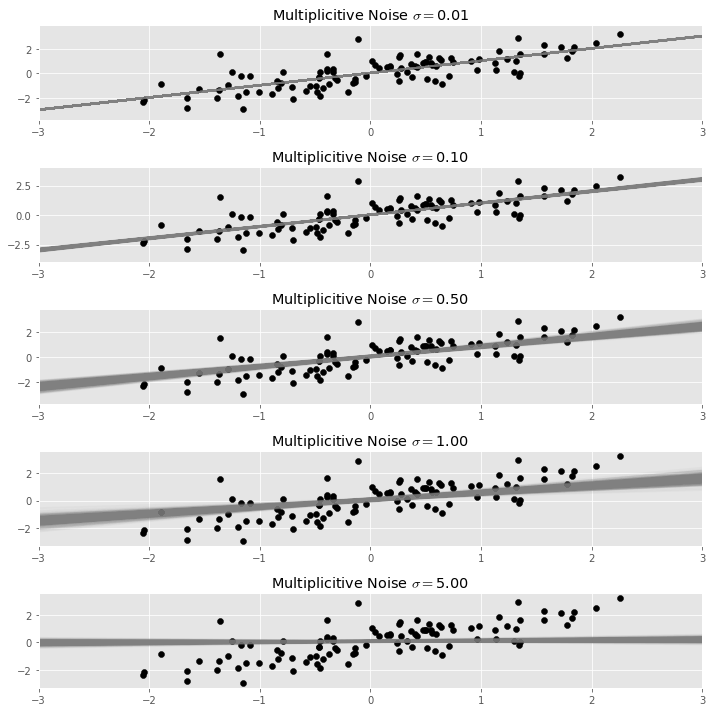
- We could average together all of our estimated regression lines. We call this average line taken over many random dispersions of the same data set the averaged regression line with noise $\sigma$.
- We could repeat the process of applying multiplicative noise multiple times, concatenate the resulting datasets, and then fit a single regression line to the inflated data. We call this single regression line fit to noisily replicated data the noise-augmented regression line with noise $\sigma$.
Below we repeat the process of applying noise and fitting a regression many times, and plot each resulting regression line. The result is a bundle of regression lines, and averaging these would produce the averaged regression line:
The noise-augmented regression line instead concatenates multiple copies of data after applying the noise repeatedly and independently, and then fits a single regression line:
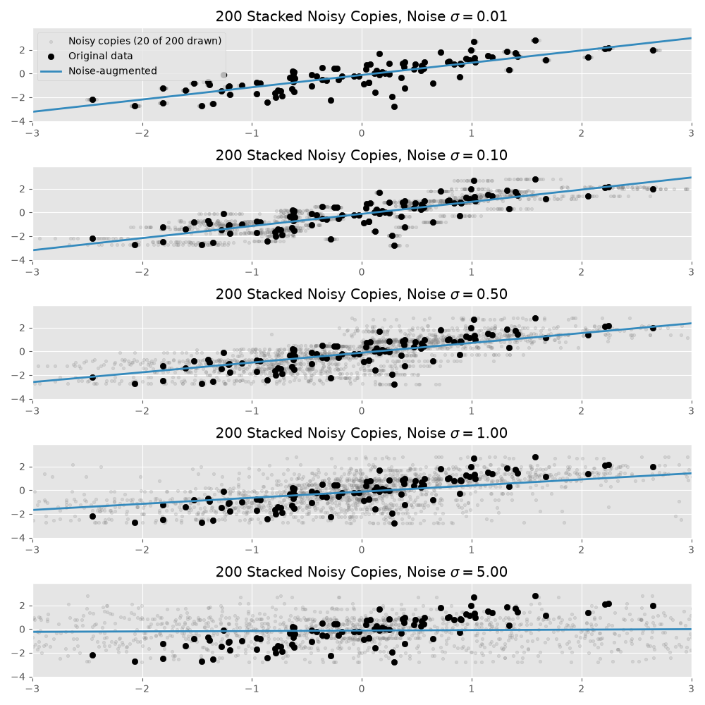
It’s tempting to think that these two ideas are really the same, that in the limit the averaged regression line is the same as the noise-augmented regression line, but they are not. The difference is small, and would not be spotted by eye unless you know what to look for. We’ll return to this point later.
Anyway, the main conclusion of this post is that one of these two procedures is equivalent to ridge regression:
The noise-augmented regression line with noise $\sigma$ converges to the ridge regression line with penalty parameter $\lambda = N \sigma^2$; here $N$ is the number of observations in the data set.
This gives yet another characterization of ridge regression, it is (the limit of) the noise-augmented regression line with a properly chosen amount of multiplicative noise $\sigma$. Here is the ridge regression superimposed on the noise-augmented line:
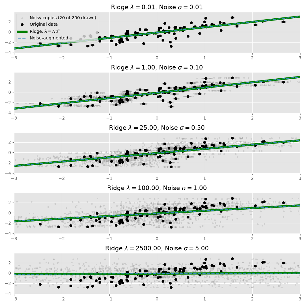
As we will now demonstrate, the lines are indistinguishable, and differ only due to sampling variance. As the number of noisy concatenated copies grows, the noise-augmented line converges to the ridge line.
The Noise-Augmented Line is the Ridge Line
In this section we give the mathematical details showing that the two regression lines are equal.
Statement of the Problem
In our setup, we scale each entry of $X$ by Gaussian noise before regressing:
where $\epsilon \sim N(1, \sigma^2)$.
Because we get a different line for each choice of random $\epsilon$, we are interested in the solution vector $\beta$ that minimizes the expected squared error, the expectation taken over the randomness in our multiplicative noise:
In this equation, $G$ represents a matrix of random Gaussian noise, the $\ast$ operator is elementwise multiplication of matrices (important: not matrix multiplication), and $E_G$ marginalizes out the contributions of the noise.
It’s likely not immediately apparent how this description maps to one or the other of our sampling then fitting procedures. Consider how one could estimate the expectation $E_G \left[ \left\lvert y - (G \ast X) \beta \right\rvert^2 \right]$ if we had some $\beta$ already in hand. Sampling noise once as $g \sim G$, we can compute the matrix $g \ast X$ and then the residual norm (squared) $\left\lvert y - (g \ast X) \beta \right\rvert^2$. This is a point estimate of the expectation, a poor one, but a point estimate nonetheless.
To improve the estimate, we can rely on the law of large numbers; we sample from $G$ repeatedly, getting $g_1, g_2, \ldots, g_K$, compute the residual norm of each, then average the results:
This is a sum of residual norms (squared). The factor of $\frac{1}{K}$ doesn’t change where the minimum is, and a sum of squared norms is itself a single squared norm, of the vectors stacked on top of each other:
So minimizing the sum is equivalent to fitting a single regression to the concatenated dataset: $K$ noisy copies of $X$ stacked together, each paired with an unchanged copy of $y$.1
Minimizing the Expectation
Let’s begin by expanding out the quantity inside the expectation:
We focus on the last term for the moment. Let’s name the random coefficient matrix $M$:
Now a single entry in this matrix is:
which in expectation is:
There are two cases here. If $i \neq j$, then $\epsilon_{ki}$ and $\epsilon_{kj}$ are independent random variables both drawn from a $N(1, \sigma^2)$, so:
When $i = j$, $\epsilon_{ki}$ and $\epsilon_{kj}$ are the same Gaussian random variable, and we can compute:
So altogether:
This means that:
Where $\mathbb{1}$ is a square matrix with a $1$ in every entry, and $\operatorname{diag}(X^t X)$ is the diagonal matrix with the same diagonal entries as $X^t X$.
Putting it All Together
Now we can compute the expectation of our entire quantity by applying the linearity of expectation, and using our previous calculation for the quadratic term:
Where $\Gamma = \sqrt{ \operatorname{diag} \left( X^t X \right) }$, the square root taken entrywise.
Overall, our original problem can be restated as
Which we recognise as linear regression with a Tikhonov regularization term. The overall regularization strength depends on the amount of noise we apply to each predictor: more noise results in stronger regularization.
Ridge Regression
To make the connection to ridge regression, we recall that in ridge regression, the predictors are conventionally standardized before regressing. That is, they are centered (so there is no intercept column to perturb with noise) and scaled so that $\frac{1}{N} \operatorname{diag}(X^t X) = I$.
If we impose this assumption on our resulting regularization problem above, we get $\Gamma = \sqrt{N} I$, and consequently:
So, under the usual assumptions of unit variance, the noise-augmented procedure is, in the limit of many noisy copies, equivalent to ridge regression with a regularization strength equal to $N \sigma^2$.
The Averaged Regression Line is not the Ridge Line
We claimed earlier that the averaged regression line with noise $\sigma$ is not the ridge line, we’ll close things out by briefly explaining why this is so.
Recall that we described the noise-augmented line as the minimizer of the expected squared error:
which relied on the law of large numbers and a data stacking argument. We showed this is equivalent to a ridge regression, which has the closed form solution:
The averaged regression line is a little easier to describe, we sample noise, fit a bundle of lines, then average those together. An individual line in the bundle solves:
So the averaged line is:
The argmin inside the expectation is a standard linear regression problem, whose solution is:
So:
And the critical point is a commonplace one: the expectation of a ratio is not the ratio of expectations.
We mentioned earlier that the difference is small, and is only observable when you know to look for it; well, now we do. Below we repeatedly draw $K$ noisy copies of the data, and compute both estimates from the same copies: the noise-augmented slope by stacking the copies and fitting once, and the averaged slope by fitting each copy and averaging. With a single copy ($K=1$) the two agree, but as $K$ grows each settles toward its own limit: the noise-augmented slopes close in on the ridge slope, while the averaged slopes settle slightly above it.
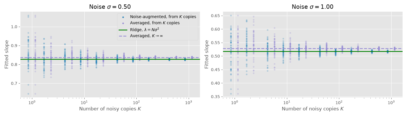
The gap is small, and shrinks as the data set grows. This can be analyzed, a second order expansion of the expectation shows that the difference between the averaged and ridge slopes shrinks like $1/N$. A detailed analysis of the difference in these estimators takes us far from our original goal, which was only to demonstrate the equivalence of ridge to the noise-augmented line. We’ll leave a more thorough elaboration for another day.
This observation and I go way back, I first encountered essentially the exact same point many years ago in a different context: Is the true linear regressor equal to the average linear regressor?2. Years later, I’m very confident that the answer to my question is no.
-
Strictly, the law of large numbers only tells us the average converges to the expectation for each fixed $\beta$, and we need the minimizers to converge too. Here that takes just a little more effort: the averaged objective is quadratic in $\beta$, with coefficients like $\frac{1}{K} \sum_i (g_i \ast X)^t (g_i \ast X)$ that are themselves sample means. Those converge to their expectations, and so the minimizer converges to the minimizer of the expected objective. ↩
-
I joined Cross Validated to ask this question. ↩