Mean Reverting Time Series and Subtle Mistakes

Danger always stalks the data analyst: whereas a software engineer’s code may fail to compile or pass unit tests, the data analyst’s work is silent about its incorrectness. It’s rare for the conclusions of an analysis of observational data to be falsifiable. This post is about a data analytic error that I’ve encountered a few times in my career.

Setup

Imagine a world with two nations:

• The Tourmekian Empire, with its currency ₮.
• The Valley of the Wind, with its currency ₩.

The nations exist in peaceful times, long after the forests have subsided and the earth cleansed of the residual toxins of war. The world has healthy culture of travel and trade.

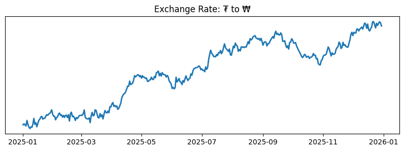
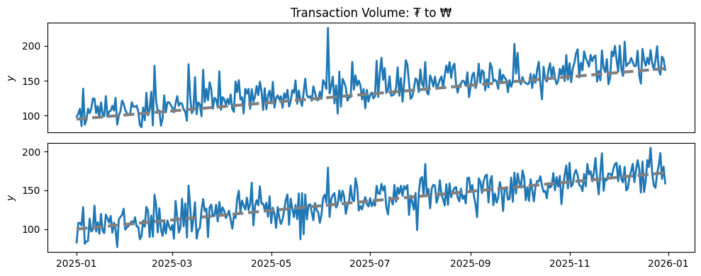
We are employed as a data analyst at a currency trading firm, our job is to support Tourmekians seeking to purchase ₩ with ₮, and Valleyers seeking to purchase ₮ with ₩. We look at plots like this, the exchange rate from ₮ to ₩, all days of our working life ¹:

At some point, a curiosity strikes us: possibly some of our customers are residents of Tourmekia, but are native to the Valley of the Wind. It’s likely some of these are using our service to exchange their Tourmekian salaries for the Valley’s ₩, with the intention of using that ₩ whenever they return to the homeland. These customer’s likely have no need to immediately make this exchange as soon as they are paid in ₮, but instead will wait for favorable moments. We hypothesize: it’s likely that exchange rate increases should associate with more usage of our service, and vice versa.

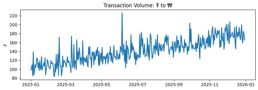
Being a responsible business that would never, ever cut corners on data engineering, we have historical data on daily transaction volumes:

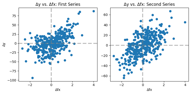
We can inspect our hypothesis by scattering the day-over-day change in transaction volume against the change in exchange rate. There is a clear association:

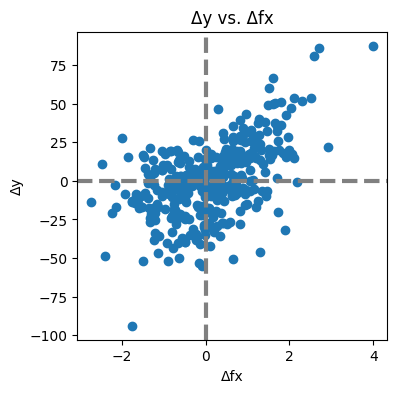
It’s simple to validate this non-visually, the mean change in volume is positive when the exchange rate increases, and negative when it decreases. Demand goes up and down in synchronization with the exchange rate. The effect is symmetric, or close enough to believe that it is:

up = df["y"].diff().filter(df["Δfx"] > 0).mean()
print(f"mean(Δy) where Δfx > 0: {up:2.2f}")
# mean(Δy) where Δfx > 0: 9.29

down = df["y"].diff().filter(df["Δfx"] < 0).mean()
print(f"mean(Δy) where Δfx < 0: {down:2.2f}")
# mean(Δy) where Δfx < 0: -10.62

This is a nice result! Our curiosity has been rewarded, and we’ve made a useful discovery about our customer dynamics. We’re wrong.

The Two Worlds

Here is a different simulation of the transaction volume series:

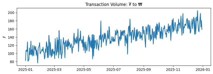
This series looks structurally identical to previous one to the untrained eye, any observer would be forgiven to allocate the slight differences to noise. In support, the summary statistics of this new series are very similar to the previous:

up = df["y_new"].diff().filter(df["Δfx"] > 0).mean()
print(f"mean(Δy) where Δfx > 0: {up:2.2f}")
# mean(Δy) where Δfx > 0: 8.97

down = df["y_new"].diff().filter(df["Δfx"] < 0).mean()
print(f"mean(Δy) where Δfx < 0: {down:2.2f}")
# mean(Δy) where Δfx < 0: -10.20

These two transaction processes are not the same, and encode very different dynamics of customer behaviour. If we scatterplot side by side, maybe the observant and lucky among us will start to sense something is up²:

We generated data according to the following random processes:

First series, asymmetric:

Second series, symmetric:

In the first scenario, the effect is not symmetric, while in the second it is symmetric. Customers in the first scenario do increase their transaction rate when the exchange rate moves favorably, but do not decrease their transaction rate when it moves against their favor.

This is much easier to see if we plot the true trendline (i.e. the $a + b t$ part of the above equations) along with our observed data series:

In the first series, the observed transaction volume mostly stays above the true trendline, any dips below are due to the noise term $\epsilon$. The second series moves around the trendline symmetrically.

So why, in the first case of only upwards effects, does our data analysis detect an association? Our finding is due to mean reversion: when the exchange rate decreases customer behaviour reverts to its baseline state of a random perturbation around the true trendline. When such an observation follows one where the exchange rate moved upwards (which happens about half the time) this results in (most likely) a downwards move from its elevated state back towards the trendline. So, on average, a fall in exchange rate is simultaneous with a fall in transaction rate.

Capturing the True Effect

Asymmetric effect are common in practice, and are worth considering whenever analysing a response to some stimuli that may be positive or negative.

The basic technique is to specify a regression model including hinge transformations of $\Delta \fx$:

If we fit this model:

X = np.column_stack([
    df["day"], 
    np.maximum(df["fx"].diff(1), 0),
    np.minimum(df["fx"].diff(1), 0),
])

regression = LinearRegression().fit(X[1:], df["y"][1:])

print(f"Regression Coefficient: β0 = {regression.intercept_:2.2f}")
# Regression Coefficient: β0 = 94.58
print(f"Regression Coefficient: βt = {regression.coef_[0]:2.2f}")
# Regression Coefficient: βt = 0.21
print(f"Regression Coefficient: β+ = {regression.coef_[1]:2.2f}")
# Regression Coefficient: β+ = 19.82
print(f"Regression Coefficient: β- = {regression.coef_[2]:2.2f}")
# Regression Coefficient: β- = -0.57

We infer correct coefficients from the observed data. In particular, we correctly deduce that there is no effect of downwards movements in $\Delta fx$.

If instead we fit the wrong model:

We infer an symmetric effect of half the size:

X = np.column_stack([
    df["day"], 
    df["fx"].diff(1)
])

regression = lin.LinearRegression().fit(X[1:], df["y"][1:])

print(f"Regression Coefficient: β0 = {regression.intercept_:2.2f}")
# Regression Coefficient: β0 = 103.16
print(f"Regression Coefficient: βt = {regression.coef_[0]:2.2f}")
# Regression Coefficient: βt = 0.20
print(f"Regression Coefficient: β = {regression.coef_[1]:2.2f}")
# Regression Coefficient: β = 10.62

Insidiously, with the wrong model we draw two incorrect conclusions: we infer half of the correct positive effect, and a negative effect when there is none.