Adding Noise to Regression Predictors is Ridge Regression

Ridge penalization is a popular and well studied method for reducing the variance of predictions in regression. There are many different yet equivalent ways to think about Ridge regression, some of the well known ones are:

• A penalized optimization problem.
• A constrained optimization problem.
• A linear regression with an augmented data set.
• A maximum a-posteriori estimate in Bayesian linear regression.

In this post we will give another, less common, characterization of ridge regression.

Software

The code used to produce the simulations and plots in this post is available in this git repository.

Acknowledgements

The idea for this post was inspired by a small section in the paper: Dropout: A Simple Way to Prevent Neural Networks from Overfitting.

Ridge Regression

Consider the usual linear regression setup.

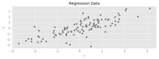
In linear regression, we seek a vector $\hat \beta$ which solves the following optimization problem:

$$\hat \beta = \operatorname{argmin}_\beta \left| y - X \beta \right|^2$$

The goal of the problem is to produce a linear function that can be used to predict new values of $y$ when only provided with values of $X$. After solving the problem and obtaining $\hat \beta$, these predicted values are given by

$$\hat y = X \hat \beta$$

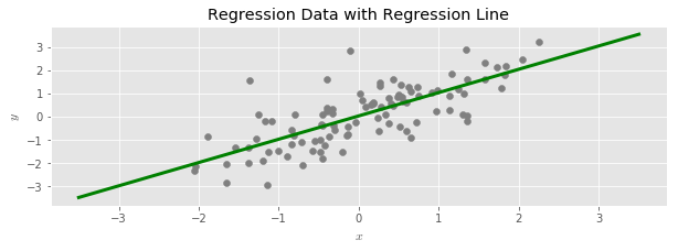
Ridge Regression is an alternate way to estimate the regression line that is useful when linear regression produces predicted values with a high variance (for example, when there is not enough data available to accurately estimate effects for all of the available predictors). Ridge often has the desirable effect of improving the predictive power of a regression.

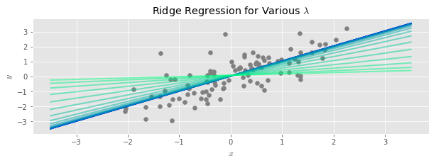
In the standard description, ridge regression is described as a penalized optimization problem:

$$\hat \beta = \operatorname{argmin}_\beta \left| y - X \beta \right|^2 + \lambda \left| \beta \right|^2$$

The parameter $\lambda$ controls the severity of the variance reduction: larger values result in more biased but lower variance estimates.

Adding Noise to Regression Predictors

In this post we will give an alternative description of ridge regression in terms of adding noise to the data used to fit a regression, and then marginalizing over the added noise by averaging together all the resulting regression lines.

Suppose we have available an unlimited number of independent and equally distributed Gaussian random variables:

$$\epsilon_1, \epsilon_2, \ldots \sim Normal(1, \sigma)$$

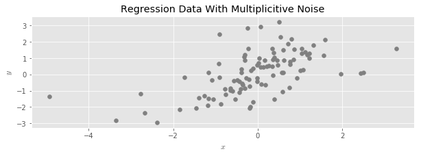
If $X$ is a matrix containing the values of features in a regression problem, we say we have added multiplicitive random noise to X when we replace $X$ with a new dataset:

$$x_{ij} \rightarrow \epsilon_{ij} x_{ij}$$

In words, we draw a random $Normal(1, \sigma)$ for every data element in $X$, and then multiply each data element by its corresponding random number.

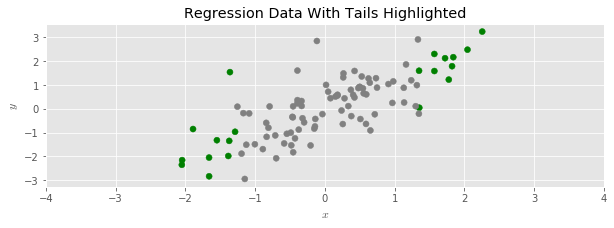
To see the effect more clearly, let’s color the upper and lower 10’th percentiles of the example regression data set:

And then disperse the data with multiplicative random noise:

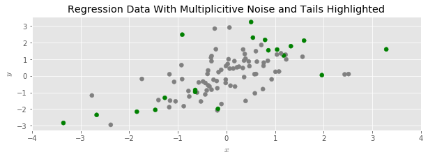
We see that the data has spread out, and its range has expanded; around half of the shaded points moved further away from the center of the point cloud.

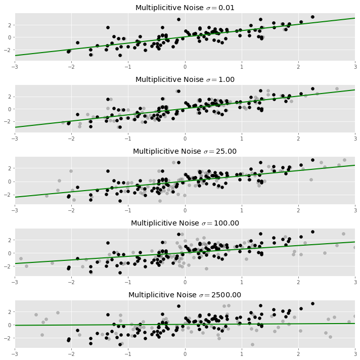
Our idea is to fit a linear regression, but to the manipulated data. Since the addition of the multiplicative noise tends to spread the point cloud out, this depresses the slope of the regression line, exactly as in ridge regression.

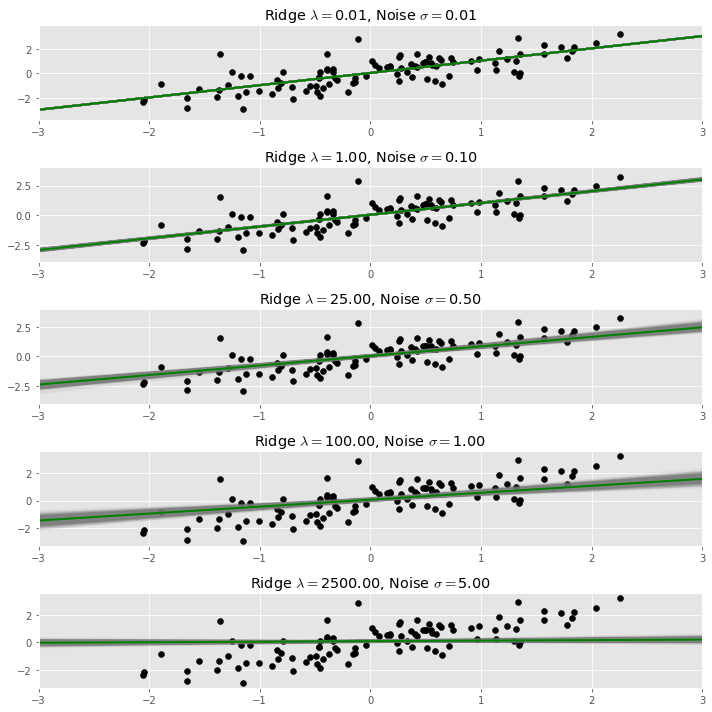
In the plot below, the original data set is plotted in black, and the dispersed data we used to fit the regression line is plotted in light grey. As more noise is added, the regression line indeed flattens.

Of course, when adding random noise to data, one expects to get a different result each time. In our case, each time we fit a regression line to a different version of our noisy data, we expect to get a slightly different line. To get a stable result out of this process, we need to average together all of our estimated regression lines. This process is called marginalization, i.e., integrating out the randomness in the process.

Below we repeat the process of adding noise and fitting a regression many times, and plot each resulting regression line. The result in a bundle of regression lines, which we can see fan out around an average line, which is the stable result of the process.

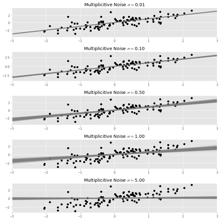
We call this average line taken over many random dispersions of the same data set the dispersed regression line with noise $\sigma$.

The main conclusion of this post is that

The dispersed regression line with noise $\sigma$ is equal to the ridge regression line with penalty parameter $\lambda = N \sigma^2$; here $N$ is the number of observations in the data set.

This gives yet another characterization of ridge regression, it is a dispersed regression line with a properly chosen amount of multiplicative noise $\sigma$.

Below we superimpose the result of a ridge regression upon our bundle of regression lines plot from above. The ridge penalty is chosen using the formula quoted above, and is shown in dark green.

Proof of The Claim

In this section we give the mathematical details showing that the two regression lines are equal.

Statement of the Problem

In our setup, we scale each entry of $X$ by a small amount of Gaussian noise before regressing:

$$x_{ij} \rightarrow \epsilon_{ij} x_{ij}$$

where $\epsilon \sim N(1, \sigma)$.

Because we get a different line for each choice of random $\epsilon$; we are interested in what happens on average. That is, we are interested in the solution vector $\beta$ that is the expectation under this process

$$\hat \beta \sim \operatorname{argmin}_\beta E_G \left[ \left| y - (G * X) \beta \right|^2 \right]$$

In this equation, $G$ represents a matrix of random Gaussian noise, the $\ast$ operator is elementwise multiplication of matrices, and $E_G$ marginalizes out the contributions of the noise.

Let’s begin the demonstration by expanding out the quantity inside the expectation:

$$\begin{align*} \left| y - (G * X) \beta \right|^2 &= \left( y - (G * X) \beta \right)^t \left( y - (G * X) \beta \right) \\ &= y^t y - 2 y^t (G * X) \beta + \beta^t (G * X)^t (G * X) \beta \end{align*}$$

Computing the Quadratic Term

We focus on the last term for the moment. Let’s name the random coefficient matrix $M$:

$$M = (G * X)^t (G * X)$$

Now a single entry in this matrix is:

$$m_{ij} = \sum_{k} \epsilon_{ki} \epsilon_{kj} x_{ki} x_{kj}$$

which in expectation is:

$$E \left[ m_{ij} \right] = \sum_{k} E \left[ \epsilon_{ki} \epsilon_{kj} \right] x_{ki} x_{kj}$$

There are two cases here. If $i \neq j$, then $\epsilon_{ki}$ and $\epsilon_{kj}$ are independent random variables both drawn from a $N(1, \sigma)$, so:

$$E \left[ \epsilon_{ki} \epsilon_{kj} \right] = 1 \text{ for } i \neq j$$

When $i = j$, the $\epsilon$s are not independent, but we can compute:

$$E \left[ \epsilon_{ki}^2 \right] = E \left[ (\epsilon_{ki} - 1)^2 + 2 \epsilon_{ki} - 1 \right] = \sigma^2 + 2 - 1 = \sigma^2 + 1$$

So altogether:

$$E \left[ \epsilon_{ki} \epsilon_{kj} \right] = \begin{cases} \sigma^2 + 1 & \text{if} \ i = j \\ 1 & \text{otherwise} \end{cases}$$

This means that

$$E[M] = \left( \mathbb{1} + diag(\sigma^2) \right) * X^t X = X^t X + diag(\sigma^2) X^t X$$

Where $\mathbb{1}$ is a square matrix with a $1$ in every entry.

Putting it All Together

Now we can compute the expectation of our entire quantity by applying the linearity of expectation, and using or previous calculation for the quadratic term:

$$\begin{align*} E \left[ \left| y - (G * X) \beta \right|^2 \right] &= E \left[ y^t y - 2 y^t (G * X) \beta + \beta^t (G * X)^t (G * X) \right] \\ &= y^t y - 2 y^t (E[G] * X) \beta + \beta^t E \left[ M \right] \beta \\ &= y^t y - 2 y^t X \beta + \beta^t X^t X \beta + \beta^t diag(\sigma^2) X^t X \beta \\ &= \left| y - X \beta \right|^2 + \beta^t diag(\sigma^2) X^t X \beta \\ &= \left| y - X \beta \right|^2 + \sigma^2 \left| \Gamma \beta \right|^2 \end{align*}$$

Where $\Gamma = \sqrt{ diag \left( X^t X \right) }$.

Overall, our original problem can be restated as

$$\hat \beta \sim \operatorname{argmin}_\beta \left( \left| y - X \beta \right|^2 + \sigma^2 \left| \Gamma \beta \right|^2 \right)$$

Which we recognise as linear regression with a tikhonov regularization term, with the overall regularization strength depending on the amount of noise we add to each predictor: more noise results in stronger regularization.

Ridge Regression

To make the connection to ridge regression, we recall that in ridge regression, we always ensure that our predictors are standardized before regressing. That is, we ensure that $\frac{1}{N}diag(X^t X) = I$.

If we impose this assumption to our resulting regularization problem above , we get $\Gamma = NI$, and consequently:

$$\hat \beta \sim \operatorname{argmin}_\beta \left( \left| y - X \beta \right|^2 + N \sigma^2 \left|\beta \right|^2 \right)$$

So, under the usual assumptions of unit variance, our add-noise procedure is in expectation equivalent to ridge regression with a regularization strength equal to $N \sigma^2$.