A Comparison of Basis Expansions in Regression

Beginners in machine learning often write off regression methods after learning of more exotic algorithms like Boosting, Random Forests, and Support Vector machines; why bother with a linear method when powerful non-parametric methods are readily available?

It’s easy to point out that the linear in linear regression is not meant to convey that the resulting model predictions are linear in the raw feaures, just the estimated parameters! The modeler can capture non-linearities in their regression, they only need to transform the raw predictors!

A common response is that the process of feature engineering is error prone, has no definite goal, and that it can be annoying work to explore data by hand and somehow divine correct transformations of predictors: why bother when other methods do it automatically.

Yet regression offers advantages that more high-tech methods do not. It is simple, and hardly a black box. Simple and common assumptions allow the modeler to perform statistical inference. It has many generalizations that advance both goals of predictive and inferential power simultaneously. And, more mundanely, it has a long history and solid foothold in many industries and sciences. Because of all this, we should seek to use this tool more skillfully.

It would be wise for us to seek a more non-parametric way to capture non-linear effects in regression models. Usually the only truly flexible method beginners learn is polynomial regression. This is a real shame, because as we will demonstrate below, it is about the worst performing method available.

The purpose of this post is to spread awareness of better options for capturing non-linearities in regression models; in particular, we would like to advocate more widespread adoption of linear and cubic splines.

Software

I’ve taken the opportunity to write a small python module that is useful for using the basis expansions in this post. It conforms to the sklearn transformation interface, so can be used in pipelines and other high level processes in sklearn.

For example, to create a simple regression model using a piecewise linear spline on a single feature, we can use the following pipelining code:

from sklearn.linear_model import LinearRegression
from basis_expansions import LinearSpline

def make_pl_regression(n_knots):
    return Pipeline([
        ('pl', LinearSpline(0, 1, n_knots=n_knots)),
        ('regression', LinearRegression(fit_intercept=True))
    ])

Users of sklearn will easily be able to adapt this to more complicated examples. For examples of use, the code used to run all the experiments and create images for this post can be found in this notebook.

Acknowledgements

The idea for this post is based on my answer to hxd1011s question regarding grouping vs. splines at CrossValidated.

Basis Expansions in Regression

To capture non-linearities in regression models, we need to transform some or all of the predictors. To avoid having to treat every predictor as a special case needing detailed investigation, we would like some way of applying a very general family of transformations to our predictors. The family should be flexible enough to adapt (when the model is fit) to a wide variety of shapes, but not too flexible as to overfit before adapting itself to the shape of the signal being modeled.

This concept of a family of transformations that can fit together to capture general shapes is called a basis expansion. The word basis here is used in the linear algebraic sense: a linearly independent set of objects. In this case our objects are functions:

and we create new sets of features by applying every function in our basis to a single raw feature:

Polynomial Expansion

The most commonly, and often only, example taught in introductory modeling courses or textbooks is polynomial regression.

In polynomial regression we choose as our basis a set of polynomial terms of increasing degree¹:

This allows us to fit polynomial curves to features:

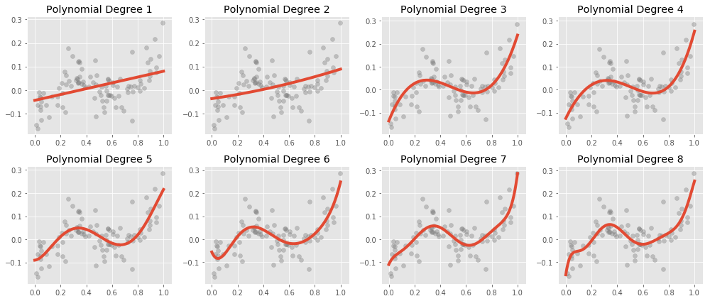
Unfortunately, polynomial regression has a fair number of issues. The most often observed is a very high variance, especially near the boundaries of the data:

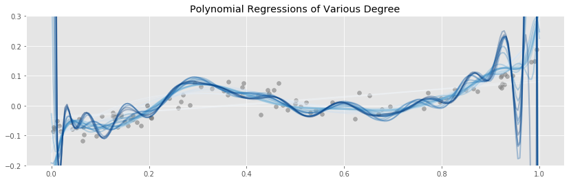
Above we have a fixed data set, and we have fit and plotted polynomial regressions of various degrees. The most striking feature is how badly the higher degree polynomials fit the data near the edges. The variance explodes! This is especially problematic in high dimensional situations where, due to the curse of dimensionality, almost all of the data is near the boundaries.

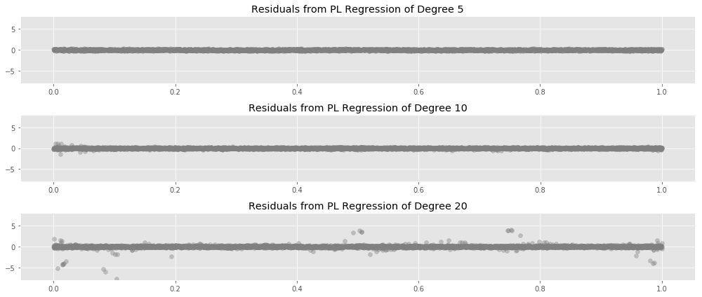
Another way to look at this is to plot residuals for each data point $x$ over many samples from the same population, as we fit polynomials of various degrees to the sampled data:

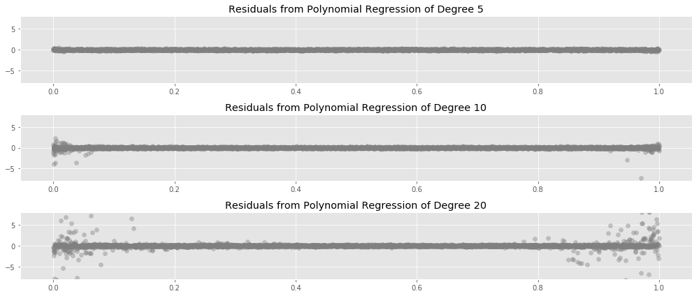
Here we see the same pattern from earlier: the instability in our fits starts at the edges of the data, and moves inward as we increase the degree.

Another final way to observe this effect is to estimate the average testing error of polynomial regressions fit repeatedly to the same population as the degree is changed:

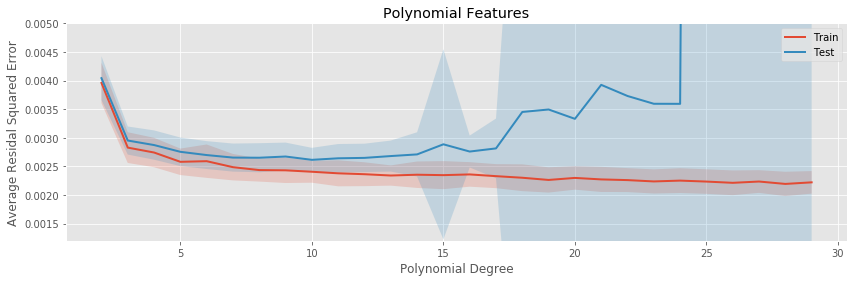
The polynomial regression eventually drastically overfits, even to this simple one dimensional data set.

There are other issues with polynomial regression; for example, it is inherently non-local, changing the value of $y$ at one point in the training set can affect the fit of the polynomial at data points very far away, resulting in tight coupling across the space of our data (often referred to as rigidity). You can get a feel for this by playing around with the interactive scatterplot somoothers app hosted on this site.

The methods we will lay out in the rest of this post will go some way to alleviate these issues with polynomial regression, and serve as superior solutions to the same underlying problems.

Binning Expansion

Probably the first thing that occurs to most modelers when reflecting on other ways to capture non-linear effects in regression is to bin the predictor variable:

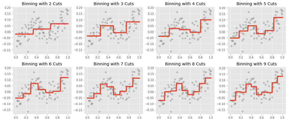
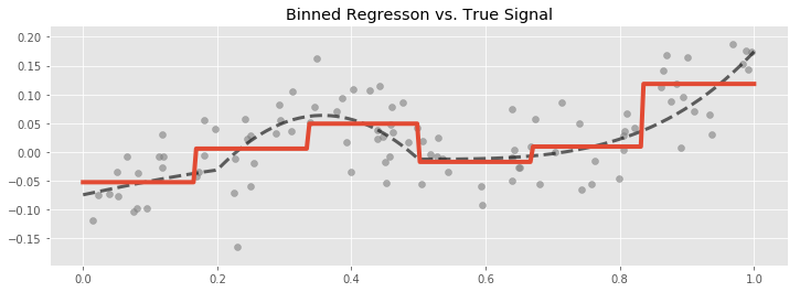
In binned regression we simply cut the range of the predictor variable into equally sized intervals (though we could use a more sophisticated rule, like cutting into intervals at percentiles of the marginal distribution of the predictor). Membership in any interval is used to create a set of indicator variables, which are then regressed upon. In the one predictor case, this results in our regression predicting the mean value of $y$ in each bin.

Binning has its obvious conceptual issues. Most prominently, we expect most phenomena we study to vary continuously with inputs. Binned regression does not create continuous functions of the predictor, so in most cases we would expect there to be some unavoidable bias within each bin. In the simple case where the true relationship is monotonic in an interval, we expect to be under predicting the truth on the left hand side of each bin, and overpredicting on the right hand side.

Even so, binning is popular. It is easy to discover, implement, and explain, and often does a good enough job of capturing the non-linear behaviour of the predictor response relationship. There are better options though, we will see later that other methods do a better job of capturing the predictive power in the data with less estimated parameters.

Piecewise Linear Splines

As a first step towards a general non-parametric continuous basis expansion, we would like to fit a piecewise linear funtion to our data. This turns out the be rather easy to do using translations of the template function $f(x) = max(0, x)$.

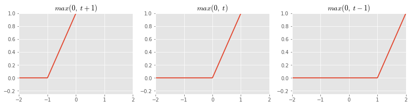
Taking linear combinations of these functions, we can create many piecewise linear shapes:

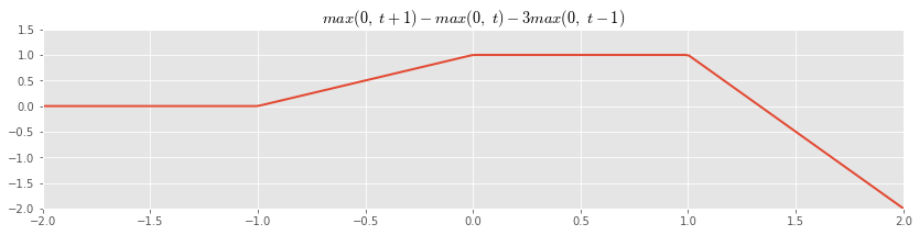
If we set down a fixed set of points where we allow the slope of the linear segment to change, then we can use these as basis functions in our regression:

The result will be to fit a continuous piecewise linear function to our data:

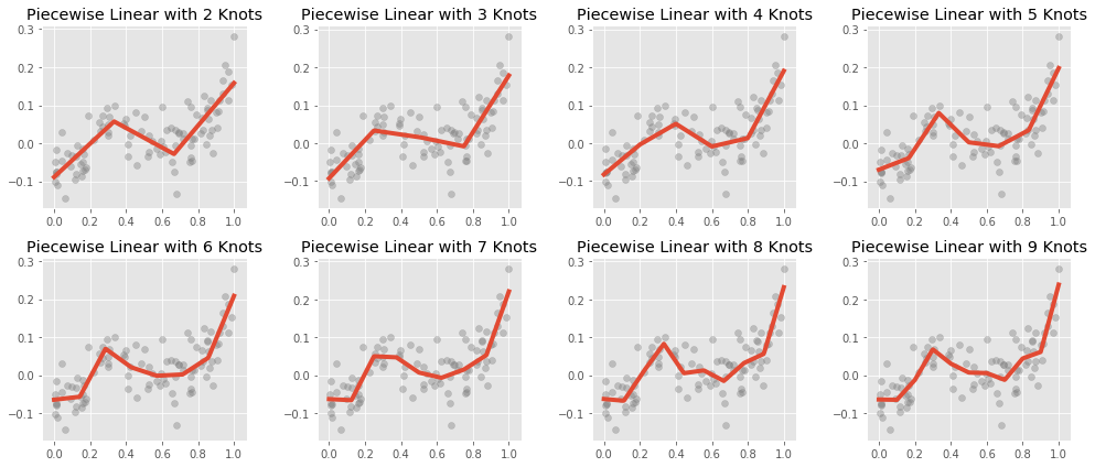
The values $\{k_1, k_2, \ldots, k_r\}$, which are the $x$ coordinates at which the slope of the segments may change, are called knots.

Note that we include the basis function $f_0(x) = x$ which allows the spline to assume some non-zero slope before the first knot. If we had not included this basis function, we would have been forced to use a zero slope in the interval $(\infty, k_1)$.

The estimated parameters for the basis function elements have a simple interpretation, they represent the change in slope when crossing from the left hand to the right hand side of a knot.

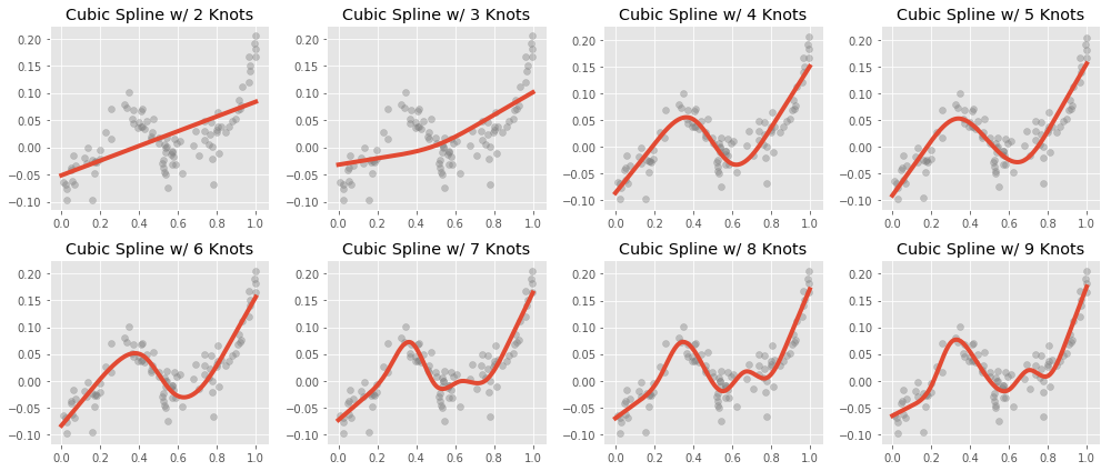
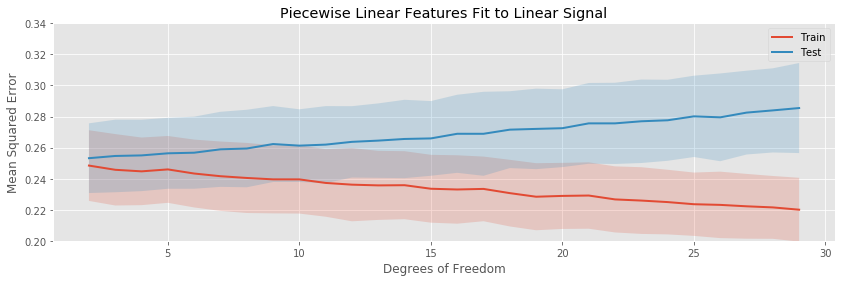
Fitting piecewise linear curves instead of polynomials prevents the explosion of variance when estimating a large number of parameters:

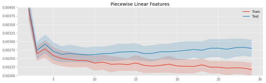
We see that as the number of knots increases, the linear spline does begin to overfit, but much more slowly than the polynomial regression with the same number of parameters.

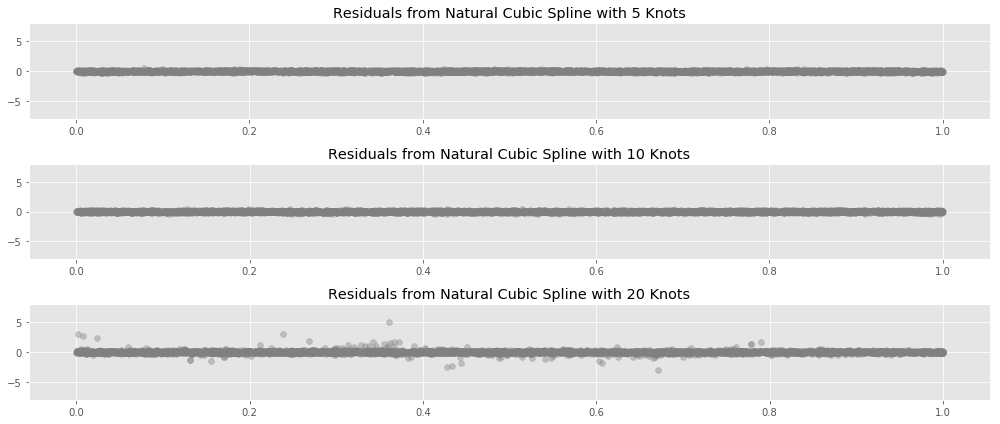
The variance does not tend to accumulate in any one area (as it did near the boundaries of the data in polynomial regression). Instead the pockets of high variance are dependent on the specific data we happen to be fitting to:

Natural Cubic Splines

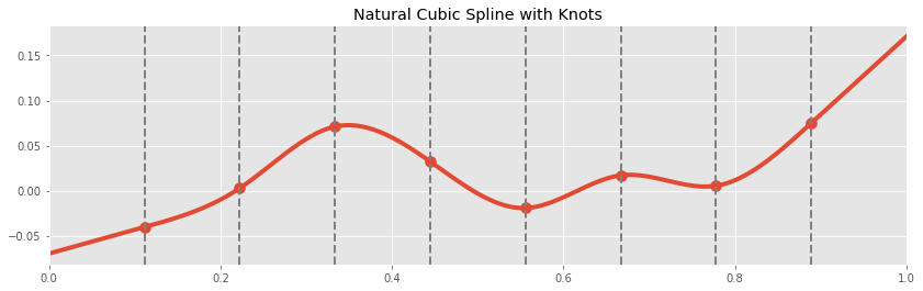
Our final example of a basis expansion will be natural cubic splines. Cubic splines are motivated by the philosophy that most phenomena we would like to study vary as a smooth function of their inputs. While the linear splines changed abruptly at the knots, we would like some way to fit curves to our data where the dependence is less violent.

A natural cubic spline is a curve that is continuous, has continuous first derivatives (the tangent line makes no abrupt changes), continuous second derivatives (the tangent lines rate of rotation makes no abrupt changes); and it equal to a cubic polynomial except a points where it is allowed to high higher order discontinuities, these points are the knots. Additionally, we require that the curve be linear beyond the knots, i.e. to the left of the first knot, and right of the final knot.

We will skip writing down the exact form of the basis functions for natural cubic spline, the interested reader can consult The Elements of Statistical Learning or the source code used in this post.

All thought they seem more complex, it is important to realize that the continuity constraints on the shape of the spline are strong. While estimating a piecewise linear spline with $r$ knots uses $r+1$ parameters (ignoring the intercept), estimating a cubic spline takes only $r$ parameters. Indeed, in the above picture, the spline with only one knot is a line; this is because the slopes of the left hand and right hand line must match.

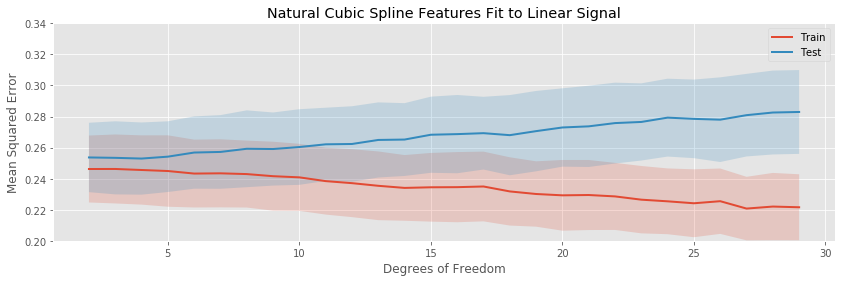
The linear constraints near the edge of the data are intended to prevent the spline for overfitting near the boundaries of the data, as polynomial regression tends to do:

Experiments

We describe below four experiments comparing the behaviour of the basis expansions above. In each experiment we fit a regression to a dataset using one of the above expansions. The degrees of freedom (number of estimated parameters) was varied, and the performance of the fit was measured on a held out dataset². This procedure what then repeated many times³ for each expansion and degree of freedom, and the average and variance of the hold out error was computed.

Our four experiments each fit to datasets sampled from a different population:

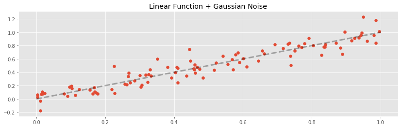
• A line plus random Gaussian noise.
• A sin curve plus random Gaussian noise.
• A weird continuous curve of mostly random design, plus random Gaussian noise.
• A sin curve with random discontinuities added, plus random Gaussian noise.

Fitting to a Noisy Line

As a first experiment, let’s fit to a linear truth. This is the simplest possible case for our regression methods, and serves to test how badly they will overfit.

Let’s look at how the training and testing error varies as we increase the number of fit parameters for each of our basis expansions

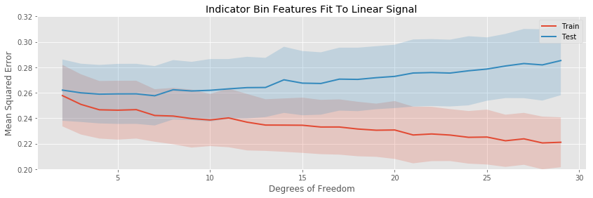
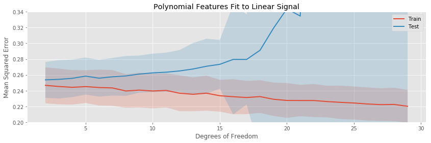
The polynomial expansion eventually overfits drastically, while the other tree transformations only overfit gradually. None of the models have any bias, so the minimum expected testing error occurs for the minimum number of fit parameters.

The binning, piecewise linear, and piecewise cubic transformations do about equally well in terms of average testing error throughout, and seem to have about the same variation in testing error (i.e. the bands around the testing error curves area ll approximately the same width).

We can get a clearer comparison by plotting only the testing errors all on the same axis:

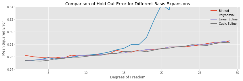
Between two and fifteen fit parameters, all the methods but polynomial regression perform about equally well, and overfit the training data at the same rate. So in this simple case, if we are only going for test performance, it doesn’t so much matter what we choose.

To examine the variance of the methods, we can plot the width of the variance bands all on the same axis:

In this example the variance of the testing error stays the same for all basis expansions throughout the entire range of complexity, with the obvious exception of polynomial regression, where the variance explodes along with the expectation.

Fitting to a Noisy Sinusoid

Our next experiment will fit the various basis expansions to a sinusoidal signal:

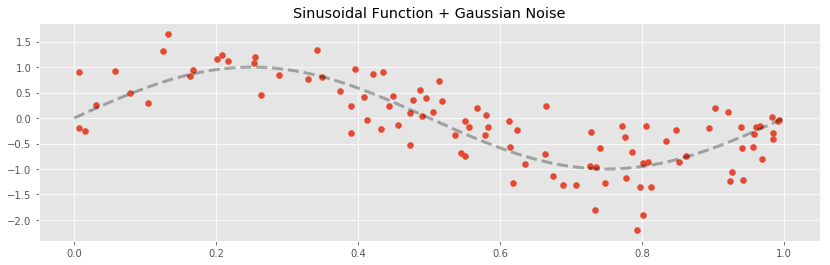
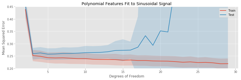
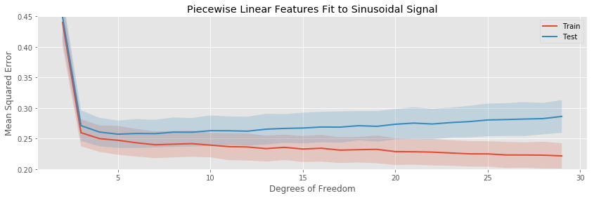
The training / testing error plots are created in the same way as for the linear signal:

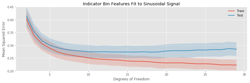
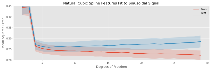
The most noticeable difference in this situation is that at a low number of estimated parameters, all the models are badly biased: while the fits to the linear function started at their lowest testing and training errors, for the sinusoid each basis expansion regression starts with high error, and decreases quickly as more parameters enter the model and the bias decreases.

The rates of overfitting tell the same story as before. The polynomial regression eventually overfits drastically, while the others overfit slowly.

Plotting the hold out error curves all on the same plot highlights another interesting feature:

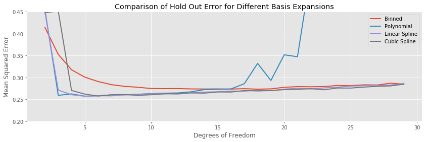
The binned regression fits to the data much more slowly than polynomial and the two splines. While the splines achieve their lowest average testing error at around five estimated parameters, it takes around eighteen bins for the binned regression to achieve its minumum. Furthermore, the minimum testing error for the polynomial and spline regressions is lower than for the bins, so we have done worse overall, but payed a higher price.

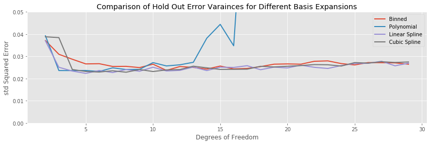
A similar story holds for the testing error variances: the binning transformation has slightly higher variance than the two spline methods.

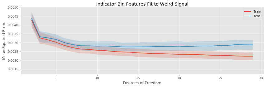
Fitting to a Noisy Weird Curve

Our next example is a weird function constructed by hand to have an unusual shape

def weird_signal(x):
    return (x*x*x*(x-1) 
            + 2*(1/(1 + np.exp(-0.5*(x - 0.5)))) 
            - 3.5*(x > 0.2)*(x < 0.5)*(x - 0.2)*(x - 0.5)
            - 0.95)

The graph of this function has exponential, quadratic, and linear qualities in different segments of its domain.

We follow the usual experiment at this point. Here are the training and testing curves for the various basis expansion methods we are investigating:

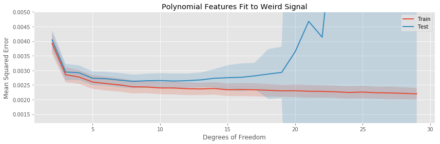
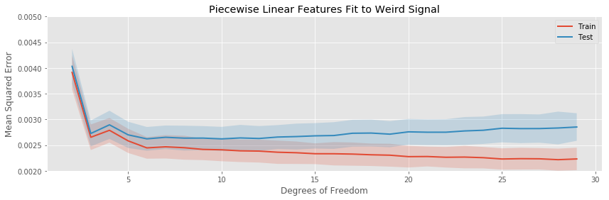
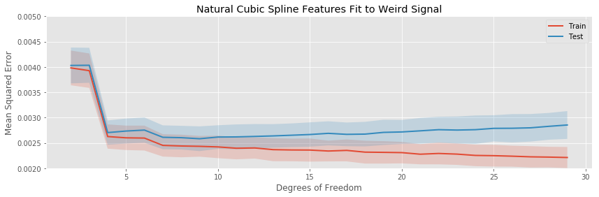
The story here captures the same general themes as in the previous example:

• The quadratic basis expansion eventually drastically overfits rapidly.
• The other basis expansions overfit slowly.
• For very a very small number of estimated parameters, each of the basis expansions is biased.
• The variance in test error is generally stable as more parameters are added to the model, except for the polynomial regression, which explodes.

Comparing all the test errors on the same plot again highlights similar points to the sin curve

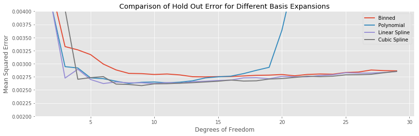
The bias of the binned regression decreases more slowly than the spline methods, and its minimum hold out error is both larger than the splines, and achieved at more estimated parameters. The linear and cubic spline generally achieve a similar testing error for the same number of estimated parameters.

The variances for the non-polynomial models are stable, with a hint that the binned regression has a larger overall variance across a range of model complexities.

Fitting to a Noisy Broken Sinusoid

For our final example, we try a discontinuous function.

cutpoints = sorted(np.random.uniform(size=6))
def broken_sin_signal(x):
    return  (np.sin(2*np.pi*x) 
             - (cutpoints[0] <= x)*(x <= cutpoints[2]) 
             - (cutpoints[1] <= x)*(x <= cutpoints[2])
             - 2*(cutpoints[3] <= x)*(x <= cutpoints[4]))

To create this function, we have taken the sin curve from before, and created discontinuities by shifting intervals of the graph up or down. The result is a broken sin curve

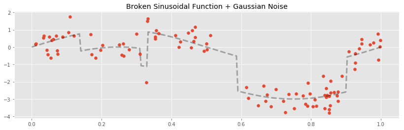
In this situation, all of our models are biased, the bins cannot capture the continuous parts correctly, while the others can not capture the discontinuities.

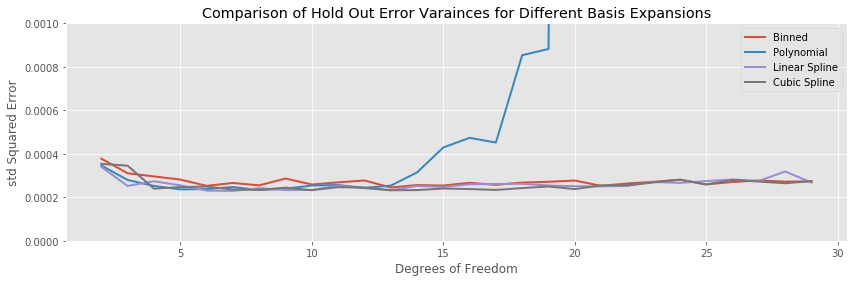
Let’s repeat our experiments and see if the discontinuities change the patterns we have been observing among the different basis expansions:

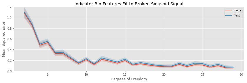
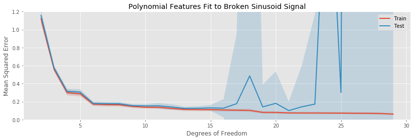
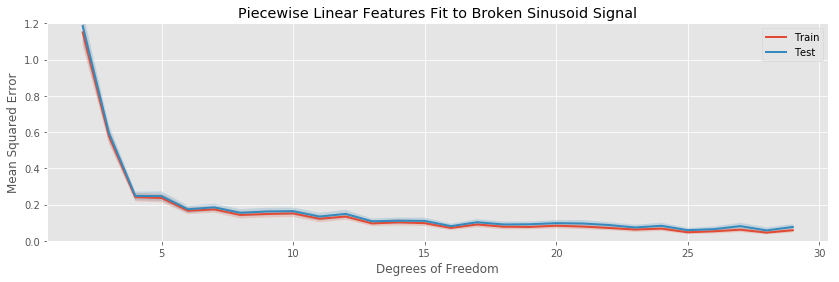
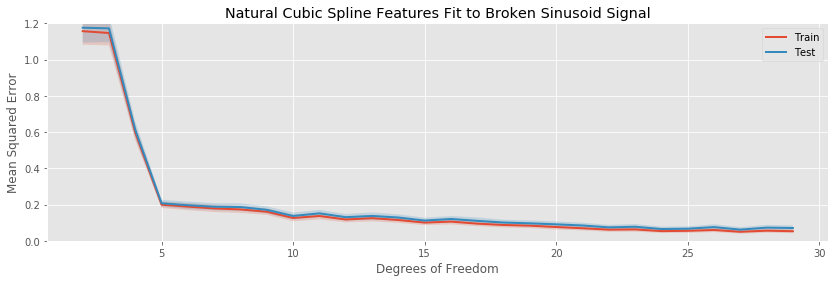
The major difference in this example is the difficulty all methods have in decreasing the bias of the fit. Since the models we are fitting are all continuous, it is impossible for any of them to be unbiased. The best we can do is trap the discontinuities between two ever closer knots (in the case of splines), or inside a small bin. Indeed, even at 29 estimated parameters, the test error is still decreasing (slowly), indicating the our models can still do a better job decreasing the bias of their fits before becoming overwhelmed with variance.

Otherwise, there are no striking differences to the patterns we observe when comparing the various basis expansions.

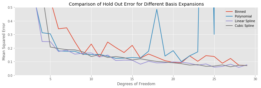
Comparing the testing errors of the various methods, this time the binned expansions does noticeably worse than the other methods throughout the entire range of complexities. Otherwise, the two spline models are mostly equivalent in performance.

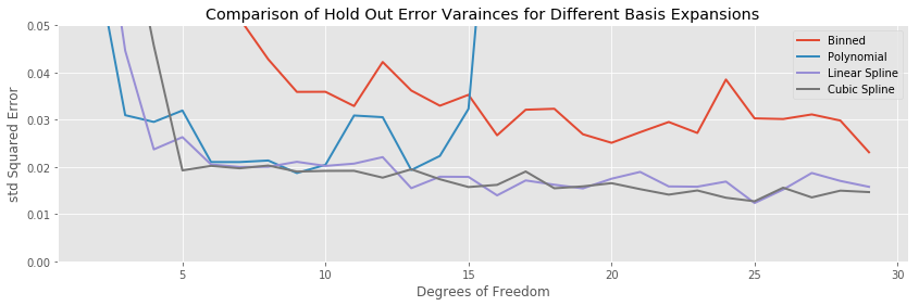
Finally, the variance of the binned model is also significantly worse in terms of variance than the other methods, while the two spline methodologies are equivalent.

Conclusions

In this post we have compared four different approaches to capturing general non-linear behaviour in regression.

Polynomial Regression

The major problem with polynomial regression is its instability once a moderate number of estimated parameters is reached. Polynomial regressions as highly sensitive to the noise in our data, and in every example were seen to eventually overfit violently; this feature was not seen in any of the other methods we surveyed.

The polynomial regression also does not accumulate variance uniformly throughout the support of the data. We saw that polynomial fits become highly unstable near the boundaries of the available data. This can be a serious issue in higher dimensional situations (though we did not explore this), where the curse of dimensionality tells us that the majority of our data will lie close to the boundary.

Binning

Binning, which conceptually simple, was seen to suffer from a few issues in comparison to the other methods

• With a small number of estimated parameters, the binned regression suffered from a higher bias than its competitors. It was seen across multiple experiments to achieve its minimal hold out error at a larger number of estimated parameters than the other methods, and furthermore, often the minimal error achieved by the binning method was larger than the minimum achieved by the other methods.
• The binned regression’s hold out error often had a higher variance than the other method’s. This means that, even if it performed just as well as another method on average, any individual binned regression is less trustworthy than if using another method.

Additionally, the binned regression method has the disadvantage of producing discontinuous functions, while we expect most processes we encounter in nature or business to vary continuously in their inputs. This is philosophically unappealing, and also accounts for some of the bias seen when comparing the binning regressions to the other basis expansions.

Linear and Cubic Splines

These methods performed well across the range of our experiments.

• They overfit slowly, especially compared to polynomial regression.
• They generally achieve a lower hold out error than the binned regressions, and achieve their minimum hold out error at a lower number of estimated parameters.
• Their hold out error is generally the lowest out of the methods we surveyed, making each individual regression more trustworthy.

The two spline models are clear winners over the binned and polynomial regressions. It is a shame that they are often not taught in introductory courses in predictive modeling. The author sees no real reason to fit polynomial or binned expansions in any predictive or inferential model, and hopes that these methods will enter the standard curriculum taught to new users of regression methods. At the very least, we hope you will use these methods in your own modeling work.